Example Cluster: Wells, Nevada
This cluster of 49 events is calibrated with the direct calibration method. Because of abundant arrival time data at very short epicentral distances for many of the events in the cluster (thanks to the temporary deployment of seismographs after the mainshock) the relocation could be done with focal depth as a free parameter for all events. This cluster also illustrates the tomo command.
From the ccat commentary file wells_summary.txt used in the GCCEL entry for this cluster:
The Wells cluster is named for the town of Wells in northeastern Nevada. The cluster is based on a mainshock-aftershock sequence that began with an Mw 5.8 event on February 21, 2008. Calibration, especially in depth, is greatly aided by data from temporary seismograph stations deployed to the source region, beginning about 2 weeks after the mainshock. The relocation was done with free depth. This cluster includes only the larger events that were located beyond local distances. For a comprehensive study, see Nealy, et al. (2017).
The run of mloc included here (wells6.1) follows from extensive work leading to publication as a journal article and also in the GCCEL database, so little further improvement is expected. The ccat command has been disabled with a comm command in the command file wells6.1.cfil, so no ~_comcat directory is created. The starting locations, empirical reading errors and spreads of phases are taken from output files of the last run of the previous series (wells5.12), which are included in the wells6 directory.
rhdf wells5.12.hdf_dcal
rfil wells5.12.rderr
tfil wells5.12.ttsprd
The wells6.1 run converged quickly to solutions very close to the starting locations, as can be seen by the small values for the change of each hypocentral parameter of the hypocentroid and the cluster vectors at each iteration. This information is a major part of the output in a ~.summary file. Here is the section on the hypocentroid from wells6.1.summary:
                         TIME        LATITUDE     LONGITUDE       DEPTH           E**2/NSTA   SHAT  PRMAX  DELT PRES FLAG
 START                12:26:17.14      41.166      -114.889        10.1

 ITER 0                      0.01 S     0.02 KM      -0.00 KM       0.30 KM      42.8/  761   1.18    4.0  8927  474 1588
 ITER 1                      0.00 S     0.01 KM       0.01 KM       0.08 KM      42.2/  761   1.17    4.0  8927  464 1588
 ITER 2                      0.01 S     0.00 KM       0.00 KM      -0.02 KM      42.0/  760   1.16    4.0  8927  465 1588

 CUMULATIVE                  0.01 S     0.04 KM       0.01 KM       0.36 KM    AZIM =    0 DEG    DIST =  0.0 KM

 SOLUTION             12:26:17.16      41.166      -114.889        10.4
 STANDARD ERRORS             0.08 S     0.002 DEG     0.003 DEG     0.98 KM    ELLIPSE:  53.3 DEG   0.4 AND    0.5 KM
The epicentroid (epicenter of the hypocentroid) shifted by only a few tens of meters and the average depth went 360 meters deeper. Since this is a direct calibration the uncertainty of the hypocentroid sets the baseline for the uncertainty of all the events; the uncertainty of the cluster vector for each event will be combined with the hypocenter’s uncertainty to obtain the final location uncertainty. The epicentroidal uncertainty seen here, 0.5 km is about as small as one ever sees for earthquake clusters relocated with standard bulletin arrival times.
Another way of reviewing how things changed is in another section of wells6.1.summary file, showing the changes in cluster vectors (overall, not by iteration). The entries for the first 10 events are:
                                       INITIAL                      CHANGE                       FINAL
 EVENT   1  20070228.1147.41     4.1 KM  AT  128 DEG          0.0 KM  AT    0 DEG          4.1 KM  AT  129 DEG
 EVENT   2  20070228.1446.10     4.2 KM  AT  136 DEG          0.0 KM  AT    0 DEG          4.2 KM  AT  137 DEG
 EVENT   3  20080221.1416.04     3.2 KM  AT  149 DEG          0.0 KM  AT    0 DEG          3.3 KM  AT  149 DEG
 EVENT   4  20080221.1420.52     4.8 KM  AT  216 DEG          0.0 KM  AT    0 DEG          4.7 KM  AT  215 DEG
 EVENT   5  20080221.1434.41     4.3 KM  AT  141 DEG          0.0 KM  AT    0 DEG          4.3 KM  AT  141 DEG
 EVENT   6  20080221.1534.25     5.0 KM  AT  207 DEG          0.0 KM  AT    0 DEG          5.0 KM  AT  207 DEG
 EVENT   7  20080221.1855.51     2.1 KM  AT  257 DEG          0.0 KM  AT    0 DEG          2.1 KM  AT  263 DEG
 EVENT   8  20080221.1906.43     4.4 KM  AT  187 DEG          0.0 KM  AT    0 DEG          4.4 KM  AT  187 DEG
 EVENT   9  20080221.1910.21     6.4 KM  AT  189 DEG          0.0 KM  AT    0 DEG          6.5 KM  AT  189 DEG
 EVENT  10  20080221.2026.08     4.1 KM  AT  241 DEG          0.4 KM  AT  341 DEG          4.1 KM  AT  246 DEG
It can be seen that event 10 moved a little bit but none of the others did, and the remaining events all show no change (within the ~50 m resolution of the output format) in epicenter during the location. Further detail is available later in wells6.1.summary, in the individual event blocks.
Free Depth
The subject of focal depth is nearly always of interest in mloc relocation studies, but when a cluster can be relocated with depth as a free parameter it is of even greater interest. One drawback of the hypocentroidal decomposition algorithm is that it places rather stringent requirements on the nature of the arrival time dataset for a free depth relocation: basically, no event can be relocated with free depth unless they all can be. If any events are poorly connected among the readings that constrain focal depth (mainly, near-source stations) the inversion will probably fail to converge. Therefore, most relocations with mloc are done with depth fixed, but there are a variety of methods to independently constrain focal depth, including free-depth relocation of a subset of events that do have data sufficient to drive a free-depth relocation.
In the version of the Wells cluster presented here, all events are stable in a free depth relocation. A review of the ~.depth_phases file shows that every event has at least 2 readings at a distance range that provides some constraint on focal depth, and most events have many more than that.
There are other output files besides wells6.1.depth_phases that bear on the evaluation of the robustness of depth determination. One very powerful tool for quickly reviewing the status is the travel-time plot for near-source readings:
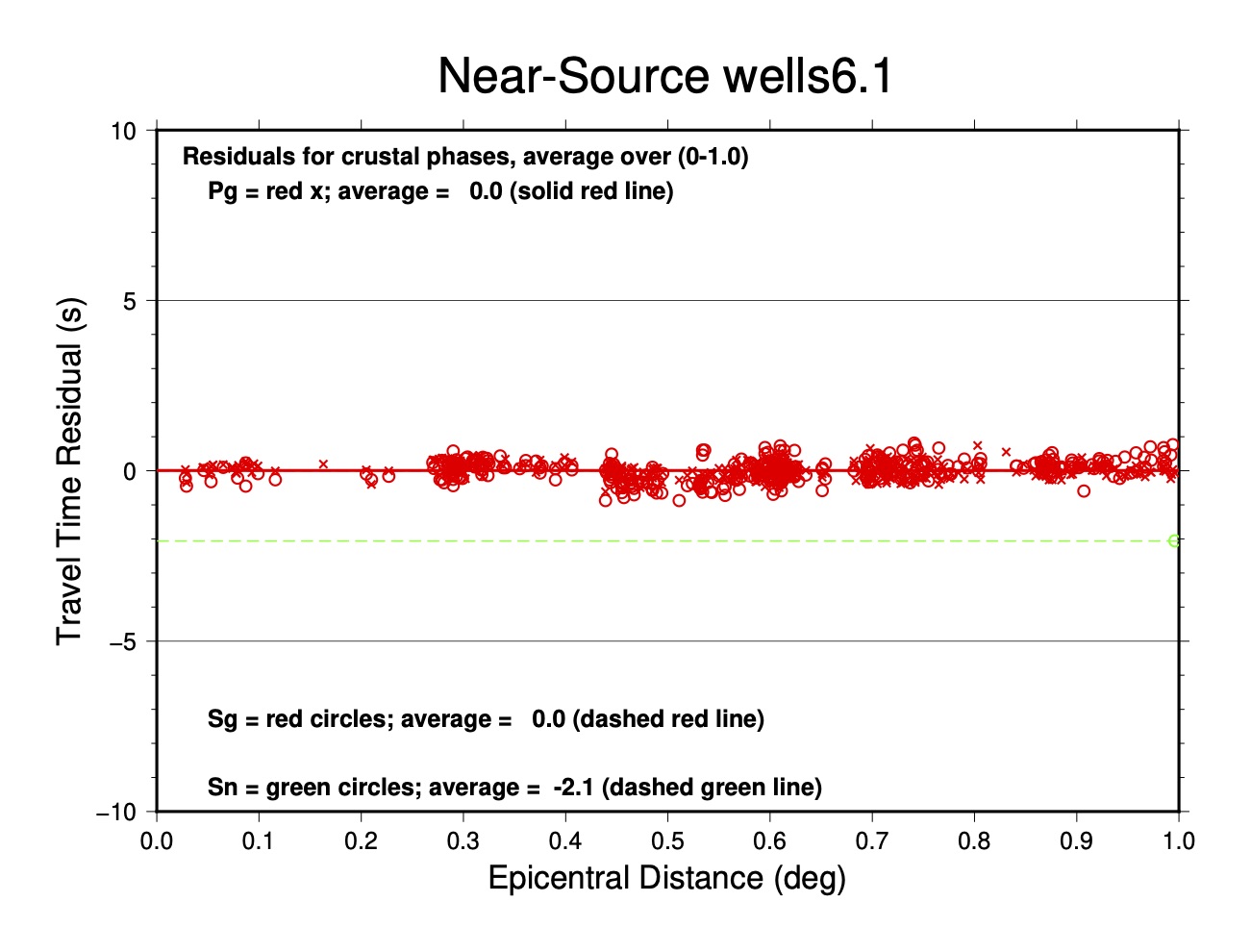
The main features we would like to see (all of which are satisfied here) are few outliers, no slope to the pattern, no curvature near zero and near-zero averages for Pg and Sg phases.
In a free-depth relocation the histogram of focal depths created by command fdhp is of special interest:
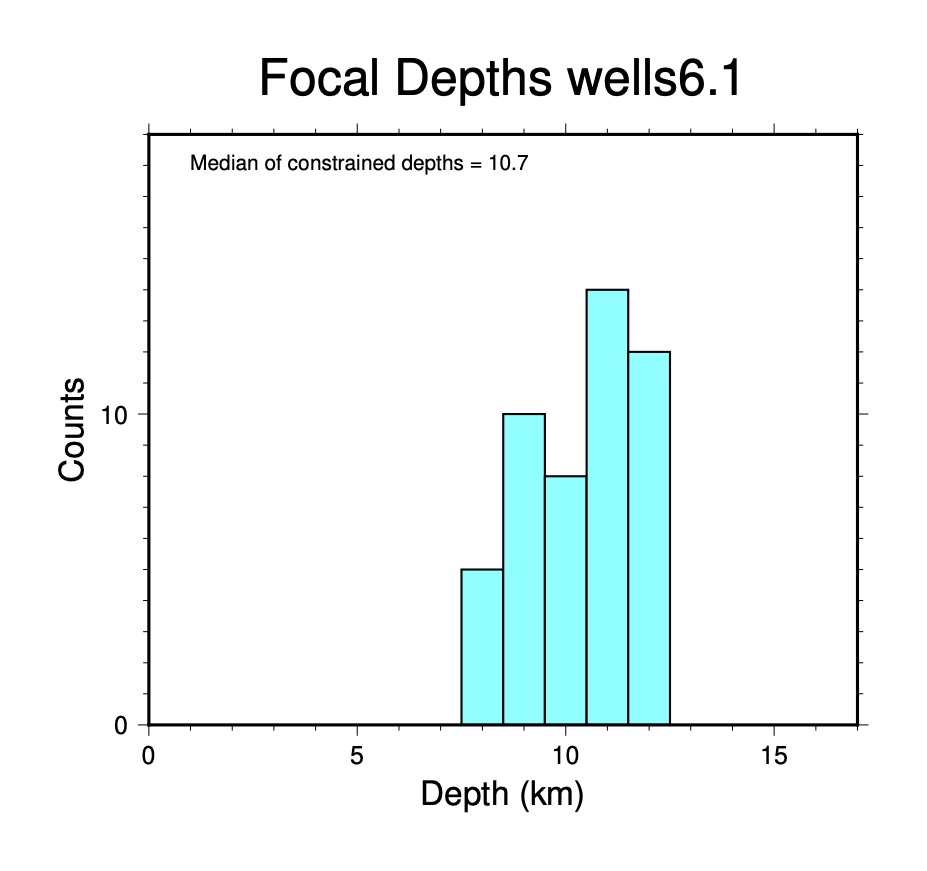
The tight pattern of resolved depths gives confidence in the results. Another aspect of this is to review the uncertainties of the depth estimates in the ~.hdf_dcal file. Here are the first 10 entries from wells6.1.hdf_dcal:
                                             Depth                                                        H+   H-
2007  2 28 11 47 40.75  41.14270 -114.85068  12.25 mf  1.60 3.4mb   11511719   16  234   34   1.00  0.14  1.1  1.1   0.3  21.4  14.6  39  0.51 129  0.56    0.9 CH01 Nevada
2007  2 28 14 46  9.51  41.13826 -114.85400  11.36 mf  4.40 3.1ML   11511822   16  169   15   1.02  0.14  1.1  1.1   0.3   6.3  16.9  40  0.52 130  0.56    0.9 CH01 Nevada
2008  2 21 14 16  2.04  41.14064 -114.86855  11.44 mf 10.00 5.8Mw   12942319    9  511   67   0.67  0.13  1.1  1.1   0.3 145.3   8.2  42  0.49 132  0.55    0.8 CH01 Nevada
2008  2 21 14 20 50.78  41.13145 -114.92061  10.68 mf 10.00 4.5mb   10542164    3   43    6   1.02  0.30  2.4  2.4   0.5 145.3  72.7  50  1.39 140  2.23    9.7 CH02 Nevada
2008  2 21 14 34 41.34  41.13560 -114.85666  12.44 mf  5.80 4.2mb   10623522   10  139   34   1.03  0.15  1.2  1.2   0.3 120.8  15.6  43  0.57 133  0.70    1.3 CH01 Nevada
2008  2 21 15 34 24.84  41.12585 -114.91570  11.05 mf 10.00 3.7mb   10623527   15  223   30   1.02  0.14  1.0  1.0   0.3 120.8  11.9  46  0.52 136  0.58    0.9 CH01 Nevada
2008  2 21 18 55 50.50  41.16363 -114.91386   9.44 mf  5.00 2.6ML   11324643   16   78    2   0.87  0.14  1.2  1.2   0.3   4.1  36.5  48  0.58 138  0.65    1.2 CH01 Nevada
2008  2 21 19  6 42.66  41.12638 -114.89507  10.09 mf 13.90 2.7ML   11324644   12   68    5   1.21  0.17  1.4  1.4   0.3   4.6  30.5  59  0.69 149  0.75    1.6 CH01 Nevada
2008  2 21 19 10 20.91  41.10845 -114.90102  11.13 mf 11.60 2.5ML   11324645   13   79    9   1.27  0.16  1.3  1.3   0.3   4.2  30.0  42  0.63 132  0.68    1.3 CH01 Nevada
2008  2 21 20 26  8.45  41.15103 -114.93307   9.44 mf  5.00 2.7ML   11324657   15   81    5   1.36  0.17  1.3  1.3   0.3   7.2  23.6  42  0.61 132  0.71    1.4 CH01 Nevada
I have added a header line to show the columns containing the converged depth and the depth uncertainty. mloc supports asymmetric depth uncertainties (“H+” and “H-“) but in a free depth solution they are the same. These values are quite good, but it can be seen that the depth constraint for event 4 is a bit weaker than others. This is likely a reflection of the fact that it has fewer readings than most, both for the connectivity through cluster vectors (43) and in the distance range used for the hypocentroid (3).
Tomography Files
In the example run of the Wells cluster the tomo command was included twice to produce output that is intended to be convenient for those conducting research in seismic tomography:
tomo Pn 3
tomo P 2
These output files are used as examples in the section on the content and format of ~.tomo files.